DeltaNet Explained (Part II)
An algorithm that parallelizes DeltaNet computation across the sequence length dimension
This blog post series accompanies our NeurIPS ‘24 paper - Parallelizing Linear Transformers with the Delta Rule over Sequence Length (w/ Bailin Wang, Yu Zhang, Yikang Shen and Yoon Kim). You can find the implementation here and the presentation slides here.
Parallel Scan for DeltaNet: A Failed Attempt
Ok, we’ve seen in the previous section that DeltaNet does really well on these diagnostic synthetic tasks. So now we just need to scale it up to modern LMs, right? Well, it turns out it’s not that simple. In particular, the original DeltaNet treated DeltaNet as a pure RNN which required O(L) sequential steps, which is inefficient on modern hardware such as GPUs with massive parallel processing capabilities. We thus seek strategies to parallelize DeltaNet across sequence length to enable hardware-efficient training. In this post, we first discuss parallel scan as a interesting-but-impractical strategy for parallelizing DeltaNet. We then give another algorithm for parallelization that is more efficient in practice.
From Delta Updates to Matrix Multiplication Form
Let’s start with DeltaNet’s original state update equation:
\[\mathbf{S}_{t} = \mathbf{S}_{t-1} - \beta_t(\mathbf{S}_{t-1} \mathbf{k}_t - \mathbf{v}_t)\mathbf{k}_t^\top\]To transform this into a matrix multiplication form, let’s expand the equation step by step:
\[\begin{align*} \mathbf{S}_{t} &= \mathbf{S}_{t-1} - \beta_t(\mathbf{S}_{t-1} \mathbf{k}_t - \mathbf{v}_t)\mathbf{k}_t^\top \\ &= \mathbf{S}_{t-1} - \beta_t \mathbf{S}_{t-1} \mathbf{k}_t \mathbf{k}_t^\top + \beta_t \mathbf{v}_t \mathbf{k}_t^\top \\ &= \mathbf{S}_{t-1} (\mathbf{I} - \beta_t \mathbf{k}_t \mathbf{k}_t^\intercal) + \beta_t \mathbf{v}_t \mathbf{k}_t^\top \end{align*}\]For simplicity, let’s denote:
- \(\mathbf{M}_t = \mathbf{I} - \beta_t \mathbf{k}_t \mathbf{k}_t^\intercal\) as our transition matrix
- \(\mathbf{X}_t = \beta_t \mathbf{v}_t \mathbf{k}_t^\top\) as our update term
Then our update becomes:
\[\mathbf{S}_{t} = \mathbf{S}_{t-1}\mathbf{M}_t + \mathbf{X}_t \in \mathbb{R}^{d\times d}\]Defining the Associative Operator
This form matches exactly with the first-order recurrence shown in equation (1.5) from Prefix Sums and Their Applications
- Matrix addition is associative: \((A + B) + C = A + (B + C)\)
- Matrix multiplication is associative: \((AB)C = A(BC)\)
- Matrix multiplication distributes over addition: \(A(B + C) = AB + AC\)
Following the framework, we define our state pairs as:
\[c_t = [\mathbf{M}_t, \mathbf{X}_t] = [\mathbf{I} - \beta_t \mathbf{k}_t \mathbf{k}_t^\intercal, \beta_t \mathbf{v}_t \mathbf{k}_t^\top]\]And our associative operator • that combines these pairs:
\[c_i \bullet c_j = [\mathbf{M}_i\mathbf{M}_j, \mathbf{M}_j\mathbf{X}_i + \mathbf{X}_j]\]This operator definition preserves the temporal dependencies of our updates - when we combine two steps, the earlier update term \(\mathbf{X}_i\) must be transformed by the later transition matrix \(\mathbf{M}_j\), while the later update term \(\mathbf{X}_j\) remains unchanged.
Parallel Scan for DeltaNet
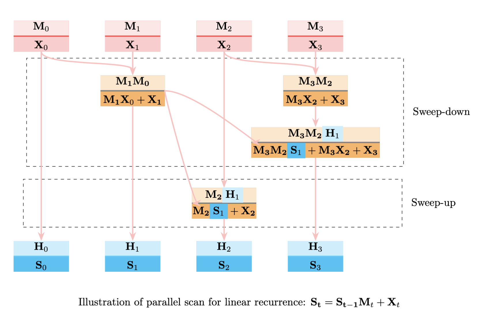
With this associative operator, we can use parallel scan to compute all states in parallel. The algorithm works in two phases:
Sweep-Down Phase
First, we compute partial results in parallel by combining adjacent pairs:
For steps 0 and 1, we compute:
\[c_1 = c_0 \bullet c_1 = [\mathbf{M}_0\mathbf{M}_1, \mathbf{M}_1\mathbf{X}_0 + \mathbf{X}_1]\]Similarly for steps 2 and 3:
\[c_3 = c_2 \bullet c_3 = [\mathbf{M}_2\mathbf{M}_3, \mathbf{M}_3\mathbf{X}_2 + \mathbf{X}_3]\]Then combine these results:
\[c_{1:3} = c_{1} \bullet c_{3} = [\mathbf{M}_0\mathbf{M}_1\mathbf{M}_2\mathbf{M}_3, \mathbf{M}_2\mathbf{M}_3(\mathbf{M}_1\mathbf{X}_0 + \mathbf{X}_1) + \mathbf{M}_3\mathbf{X}_2 + \mathbf{X}_3]\]Sweep-Up Phase
In this phase, we use our partial results to compute intermediate states:
\[c_2 = c_1 \bullet c_2 = [\mathbf{M}_1\mathbf{M}_2, \mathbf{M}_2\mathbf{X}_1 + \mathbf{X}_2]\]This parallelization transforms DeltaNet’s sequential state updates into an efficient parallel computation, reducing the sequential dependency chain from \(\mathbf{O}(L)\) to \(\mathcal{O}(\log L)\) steps while maintaining mathematical equivalence.
What’s Wrong with Parallel Scan for DeltaNet?
Despite parallelizability, parallel scan for DeltaNet faces two major challenges: computational complexity and memory requirements.
The first issue lies in the time complexity. For DeltaNet, parallel scan yields \(\mathcal{O}(L\log L d^3)\) complexity due to the cubic cost of matrix multiplication when treating \(\mathbf{M}_t\) as dense matrices. At first glance, we might think we can leverage the identity-plus-low-rank structure of \(\mathbf{M}_t\) for acceleration. Let’s work through this carefully.
When multiplying two adjacent matrices, we get:
\[\begin{align*} (\mathbf{I}-\beta_0 \mathbf{k}_0 \mathbf{k}_0^\top)(\mathbf{I} - \beta_1 \mathbf{k}_1 \mathbf{k}_1^\top) &= \mathbf{I}(\mathbf{I} - \beta_1 \mathbf{k}_1 \mathbf{k}_1^\top) - \beta_0 \mathbf{k}_0 \mathbf{k}_0^\top(\mathbf{I} - \beta_1 \mathbf{k}_1 \mathbf{k}_1^\top) \\ &= (\mathbf{I} - \beta_1 \mathbf{k}_1 \mathbf{k}_1^\top) - \beta_0 \mathbf{k}_0 \mathbf{k}_0^\top + \beta_0\beta_1 \mathbf{k}_0 \mathbf{k}_0^\top \mathbf{k}_1 \mathbf{k}_1^\top \\ &= \mathbf{I} - \beta_1 \mathbf{k}_1 \mathbf{k}_1^\top - \beta_0 \mathbf{k}_0 \mathbf{k}_0^\top + \beta_0\beta_1 \mathbf{k}_0 (\mathbf{k}_0^\top \mathbf{k}_1) \mathbf{k}_1^\top \end{align*}\]This computation reduces the complexity from \(\mathcal{O}(d^3)\) to \(\mathcal{O}(d^2)\) by leveraging the identity-plus-low-rank structure - we only need to compute vector inner products \((\mathbf{k}_0^\top \mathbf{k}_1)\) and outer products between vectors. Similarly for the next pair:
\[\begin{align*} (\mathbf{I}-\beta_2 \mathbf{k}_2 \mathbf{k}_2^\top)(\mathbf{I} - \beta_3 \mathbf{k}_3 \mathbf{k}_3^\top) &= \mathbf{I} - \beta_3 \mathbf{k}_3 \mathbf{k}_3^\top - \beta_2 \mathbf{k}_2 \mathbf{k}_2^\top + \beta_2\beta_3 \mathbf{k}_2 (\mathbf{k}_2^\top \mathbf{k}_3) \mathbf{k}_3^\top \end{align*}\]When we try to combine these results to compute larger spans like \(c_{1:4}\), the multiplication becomes increasingly complex. We need to multiply:
\[(\mathbf{I} - \beta_1 \mathbf{k}_1 \mathbf{k}_1^\top - \beta_0 \mathbf{k}_0 \mathbf{k}_0^\top + \beta_0\beta_1 \mathbf{k}_0 (\mathbf{k}_0^\top \mathbf{k}_1) \mathbf{k}_1^\top)(\mathbf{I} - \beta_3 \mathbf{k}_3 \mathbf{k}_3^\top - \beta_2 \mathbf{k}_2 \mathbf{k}_2^\top + \beta_2\beta_3 \mathbf{k}_2 (\mathbf{k}_2^\top \mathbf{k}_3) \mathbf{k}_3^\top)\]Each term in the first bracket must multiply with each term in the second bracket. While each matrix is initially a sum of \(O(1)\) rank-1 terms, this multiplication leads to a quadratic growth in the number of terms. After \(\log L\) levels of parallel scan, we end up with \(O(L^{\log c})\) terms, where \(c\) is the initial number of terms per matrix. This exponential growth in the number of terms, despite each being rank-1, makes maintaining the explicit structure impractical. Therefore, treating these as dense matrices with \(O(d^3L \log L)\) complexity becomes a more reasonable approach, especially considering the efficiency of dense matrix operations on modern hardware. This explains why parallel scan, while theoretically appealing, faces significant practical challenges for DeltaNet computation.
The second major issue is space complexity. Parallel scan requires materializing all intermediate d×d matrices at each step to high-bandwidth memory (HBM). For linear RNNs with matrix-valued states, this materialization becomes prohibitively expensive (\(\mathcal{O}(Ld^2)\)). While recurrent computation can avoid such materialization
Dear parallel-scan people.
— François Fleuret (@francoisfleuret) May 21, 2024
Q(t) and K(t) are 1xD and V(t) is 1xC, with D and T large, and I want to compute
Y(t) = Q(t)M(t)
with
M(0)=0
M(t+1) = M(t) + K(t)^T V(t)
A naive non-parallel scan approach is O(T) in time but I do not have to store any DxD
1/2
The key idea is to only materialize chunk-level hidden states, using matmuls to calculate outputs based on the query, key, and value matrices and chunk-level hidden states. This method avoids materializing the hidden state for every single timestep.
— Songlin Yang (@SonglinYang4) May 21, 2024
Here I previously discussed the chunkwise algorithm - another type of associative scan that offers improved memory efficiency and better utilization of tensor cores by enabling more matrix multiplication operations (for a detailed analysis, see
A Chunkwise Algorithm for DeltaNet
Chunkwise Parallel Form for Linear Attention
Linear attention’s efficiency stems from its ability to maintain a compact representation of the state using vectors rather than materializing full matrices. This is possible because a sum of outer products can be rewritten as matrix multiplication:
\[\begin{align*} \sum_{i=1}^t \mathbf{v}_i \mathbf{k}_i^\top &= \mathbf{V}_t\mathbf{K}_t^\top \\ \text{where } \mathbf{V}_t &= [\mathbf{v}_1, \mathbf{v}_2, ..., \mathbf{v}_t] \\ \mathbf{K}_t &= [\mathbf{k}_1, \mathbf{k}_2, ..., \mathbf{k}_t] \end{align*}\]This matrix multiplication form is highly optimized on modern GPUs with tensor cores. Leveraging this property, instead of storing all intermediate hidden states, we can store states only at regular intervals of size \(C\) as checkpoints. This gives us states \(\mathbf{S}_{0}, \mathbf{S}_{C}, \mathbf{S}_{2C}, ..., \mathbf{S}_{(n-1)C}\) where \(n = \lceil L/C \rceil\).
Denoting \(\mathbf{S}_{[i]} := \mathbf{S}_{iC} \in \mathbb{R}^{d \times d}\); \(\square_{[i]} = \square_{iC+1:(i+1)C} \in \mathbb{R}^{C \times d}\) for \(\square \in \{\mathbf{Q}, \mathbf{K}, \mathbf{V}, \mathbf{O}\}\); \(\square_{[i]}^r = \square_{iC+r}\) for \(\square \in \{\mathbf{q}, \mathbf{k}, \mathbf{v}, \mathbf{o}, \mathbf{S}\}\). For any position r within chunk i, we can compute:
\[\begin{align*} \mathbf{S}_{[i]}^r &= \mathbf{S}_{[i]} + \sum_{t=1}^{r} \mathbf{v}_{[i]}^t \mathbf{k}_{[i]}^{t\top} \\ \mathbf{o}_{[i]}^r &= \mathbf{S}_{[i]}^r \mathbf{q}_{[i]}^r = \mathbf{S}_{[i]}\mathbf{q}_{[i]}^r + \sum_{t=1}^{r} \mathbf{v}_{[i]}^t (\mathbf{k}^{t\top}_{[i]} \mathbf{q}_{[i]}^r) \end{align*}\]and in matrix form,
\[\begin{align*} \mathbf{S}_{[t+1]} &= \mathbf{S}_{[t]} + \mathbf{V}_{[t]}^\top \mathbf{K}_{[t]} && \in \mathbb{R}^{d\times d} \\ \mathbf{O}_{[t]} &= \mathbf{Q}_{[t]} \mathbf{S}_{[t]}^\top + (\mathbf{Q}_{[t]}\mathbf{K}_{[t]}^\top \odot \mathbf{M}) \mathbf{V}_{[t]} && \in \mathbb{R}^{C\times d} \end{align*}\]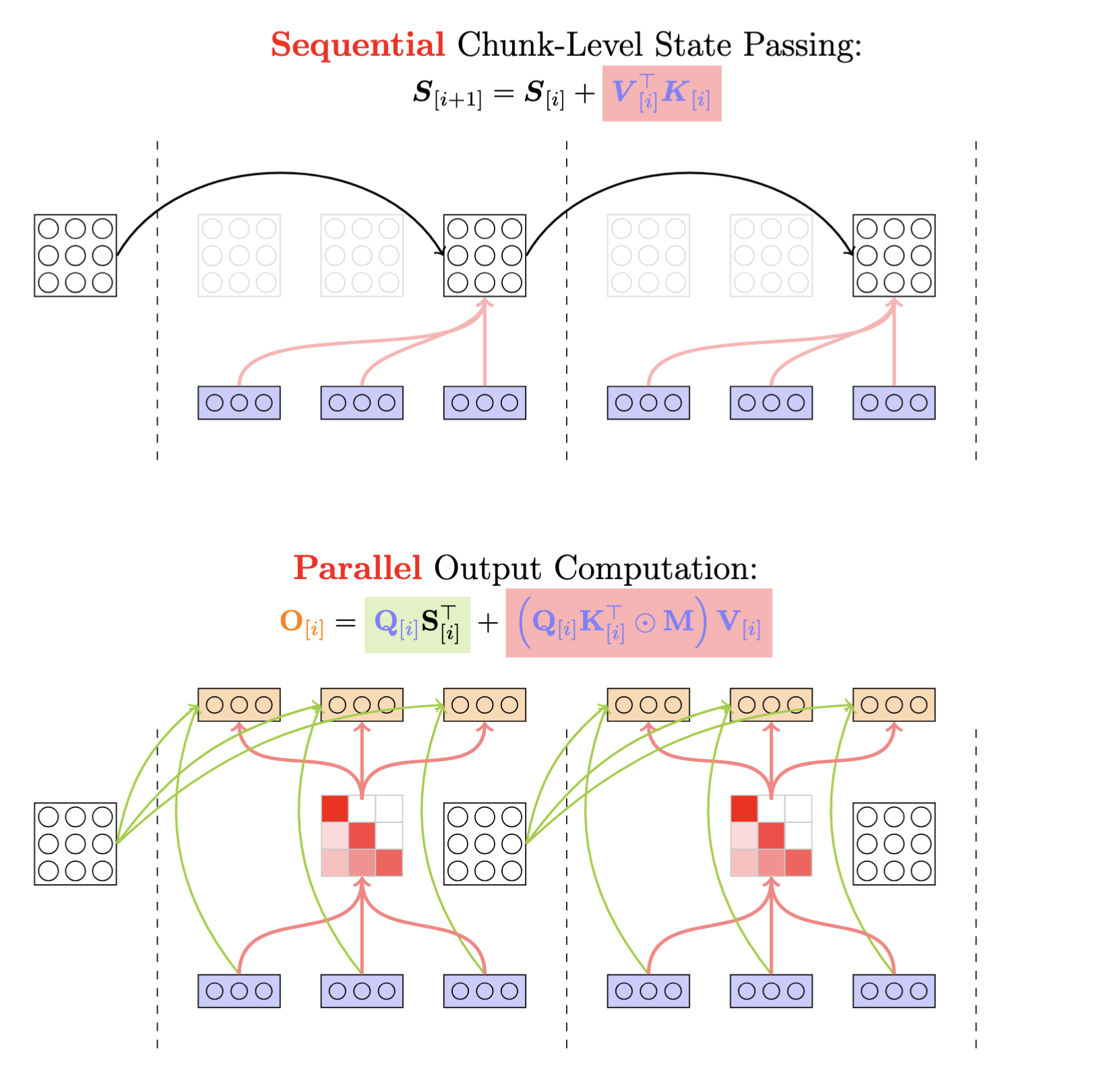
This chunkwise formulation enables efficient hardware utilization by leveraging tensor cores when the chunk size C is a multiple of 16, as implemented in our open-source library flash-linear-attention
WY representation for DeltaNet
However, as we saw in our failed attempt above, the cumulative product of DeltaNet’s transition matrices seemed to resist such compact representation, apparently requiring us to store numerous intermediate results. Fortunately, there’s a solution: DeltaNet’s transition matrices closely resemble Householder matrices (when \(\beta_t\)=2), and there exists an elegant compact representation for their cumulative product.
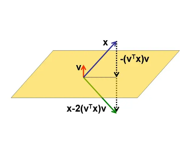
This representation, known as the WY representation, was introduced in a seminal 1985 paper
We can prove this by mathematical induction. Let’s define \(\mathbf{P}_n = \prod_{t=1}^n(\mathbf{I} - \beta_t \mathbf{k}_t \mathbf{k}_t^\top)\). For n=1, the equation clearly holds. Assuming it holds for n-1, we can prove it for n:
\[\begin{align*} \mathbf{P}_n &= \mathbf{P}_{n-1} (\mathbf{I} - \beta_n \mathbf{k}_n \mathbf{k}_n^\top) \\ &= (\mathbf{I} - \sum_{t=1}^{n-1} \mathbf{w}_t \mathbf{k}_t^\top)(\mathbf{I} - \beta_n \mathbf{k}_n \mathbf{k}_n^\top) \\ &= \mathbf{I} - \sum_{t=1}^{n-1} \mathbf{w}_t \mathbf{k}_t^\top - \beta_n \mathbf{k}_n \mathbf{k}_n^\top + (\sum_{t=1}^{n-1} \mathbf{w}_t \mathbf{k}_t^\top) \beta_n \mathbf{k}_n \mathbf{k}_n^\top \\ &= \mathbf{I} - \sum_{t=1}^{n-1} \mathbf{w}_t \mathbf{k}_t^\top - \underbrace{\left(\beta_n \mathbf{k}_n - \beta_n \sum_{t=1}^{n-1} \left(\mathbf{w}_t (\mathbf{k}_t^\top\mathbf{k}_n)\right) \right)}_{\mathbf{w}_n}\mathbf{k}_n^\top \\ &= \mathbf{I} - \sum_{t=1}^n \mathbf{w}_t\mathbf{k}_t^\top \end{align*}\]This proof not only establishes the correctness of the representation but also provides a constructive way to compute the \(\mathbf{w}\) vectors!
Similarly, we can show \(\mathbf{S}_n = \sum_{t=1}^{n} \mathbf{u}_t \mathbf{k}_t^\top\) by induction:
\[\begin{align*} \mathbf{S}_n &= \mathbf{S}_{n-1} (\mathbf{I} - \beta_n \mathbf{k}_n\mathbf{k}_n^\top) + \beta_n \mathbf{v}_n \mathbf{k}_n^\top \\ &= \left(\sum_{t=1}^{n-1} \mathbf{u}_{t}\mathbf{k}_{t}^\top\right) (\mathbf{I} - \beta_n \mathbf{k}_n\mathbf{k}_n^\top) + \beta_n \mathbf{v}_n \mathbf{k}_n^\top \\ &= \sum_{t=1}^{n-1} \mathbf{u}_{t}\mathbf{k}_{t}^\top - \left(\sum_{t=1}^{n-1} \mathbf{u}_{t}\mathbf{k}_{t}^\top\right) \beta_n \mathbf{k}_n \mathbf{k}_n^\top + \beta_n \mathbf{v}_n \mathbf{k}_n^\top \\ &= \sum_{t=1}^{n-1} \mathbf{u}_{t}\mathbf{k}_{t}^\top + \underbrace{\left(\beta_n \mathbf{v}_n - \beta_n\sum_{t=1}^{n-1} \mathbf{u}_t \left(\mathbf{k}_t^\top \mathbf{k}_n \right) \right)}_{\mathbf{u}_n} \mathbf{k}_n^\top \\ &= \sum_{t=1}^{n} \mathbf{u}_t \mathbf{k}_t^\top \end{align*}\]Looking at this sum-of-outer-products structure, we can see it closely resembles linear attention’s update form. This similarity suggests a path toward developing a novel parallel algorithm!
Chunkwise Parallel Form for DeltaNet
First, let’s unroll the recurrence of DeltaNet:
\[\begin{align*} \mathbf{S}_t &= \mathbf{S}_{t-1} (\mathbf{I} - \beta_t \mathbf{k}_t \mathbf{k}_t^\top) + \beta_t \mathbf{v}_t \mathbf{k}_t^\top \\ &= \sum_{i=1}^t \beta_i (\mathbf{v}_i \mathbf{k}_i^\top) \left(\prod_{j=i+1}^t (\mathbf{I} - \beta_j \mathbf{k}_j \mathbf{k}_j^\top)\right) \end{align*}\]Similar to linear attention, we can use checkpointing to store states at regular intervals of size C. For any position r within chunk i, we have:
\[\begin{align*} \mathbf{S}_{[i]}^r &= \mathbf{S}_{[i]} \underbrace{\prod_{t=1}^{r} (\mathbf{I}-\beta_{[i]}^t\mathbf{k}_{[i]}^t\mathbf{k}_{[i]}^{t\top})}_{\text{chunk-local cumprod: } \mathbf{P}_{[i]}^r} + \underbrace{\sum_{t=1}^{r} (\beta_{[i]}^t \mathbf{v}_{[i]}^t \mathbf{k}_{[i]}^{t\top} \prod_{s=t+1}^{r} (\mathbf{I}-\beta_{[i]}^s\mathbf{k}_{[i]}^s\mathbf{k}_{[i]}^{s\top}))}_{\text{chunk-local state or cumprodsum: }\mathbf{H}_{[i]}^r} \\ &= \mathbf{S}_{[i]} (\mathbf{I} - \sum_{t=1}^r\mathbf{w}_{[i]}^t\mathbf{k}_{[i]}^{t\top}) + \sum_{t=1}^r \mathbf{u}_{[i]}^t \mathbf{k}_{[i]}^{t\top}\\ \end{align*}\]where \(\mathbf{w}_{[i]}^t\) and \(\mathbf{u}_{[i]}^t\) are computed using the WY representation, but starting from the first position of each chunk rather than the beginning of the sequence, enabling parallel computation across chunks.
\[\mathbf{w}_{[t]}^r = \beta_{[t]}^r \left(\mathbf{k}_{[t]}^r - \sum_{i=1}^{r-1} \mathbf{w}_{[t]}^i (\mathbf{k}_{[t]}^i)^\top\mathbf{k}_{[t]}^r \right)\] \[\mathbf{u}_{[t]}^r = \beta_{[t]}^r \left(\mathbf{v}_{[t]}^r - \sum_{i=1}^{r-1} \mathbf{u}_{[t]}^i (\mathbf{k}_{[t]}^i)^\top\mathbf{k}_{[t]}^r \right)\]And for output computation,
\[\begin{align*} \mathbf{o}_{[i]}^r &= \mathbf{S}_{[i]}^r \mathbf{q}_{[i]}^r \\ &= \mathbf{S}_{[i]} \mathbf{q}_{[i]}^r - \sum_{t=1}^r \mathbf{S}_{[i]}\mathbf{w}_{[i]}^t(\mathbf{k}_{[i]}^{t\top}\mathbf{q}_{[i]}^r) + \sum_{t=1}^r \mathbf{u}_{[i]}^t(\mathbf{k}_{[i]}^{t\top}\mathbf{q}_{[i]}^r) \\ &= \mathbf{S}_{[i]} \mathbf{q}_{[i]}^r + \sum_{t=1}^r (\mathbf{u}_{[i]}^t - \mathbf{S}_{[i]}\mathbf{w}_{[i]}^t)(\mathbf{k}_{[i]}^{t\top}\mathbf{q}_{[i]}^r) \end{align*}\]Together, in matrix-multiplication form,
\[\begin{align*} \mathbf{S}_{[i+1]} &= \mathbf{S}_{[i]} (\mathbf{I}-\mathbf{W}_{[i]}^\top \mathbf{K}_{[i]}) + \mathbf{U}_{[i]}^\top \mathbf{K}_{[i]} \\ &= \mathbf{S}_{[i]} + \left(\mathbf{U}_{[i]} - \mathbf{W}_{[i]}\mathbf{S}_{[i]}^\top\right)^\top \mathbf{K}_{[i]} && \in \mathbb{R}^{d\times d} \\ \mathbf{O}_{[i]} &= \mathbf{Q}_{[i]} \mathbf{S}_{[i]}^\top + (\mathbf{Q}_{[i]} \mathbf{K}_{[i]}^\top \odot \mathbf{M}) \left(\mathbf{U}_{[i]} - \mathbf{W}_{[i]} \mathbf{S}_{[i]}^\top\right) && \in \mathbb{R}^{C\times d} \end{align*}\]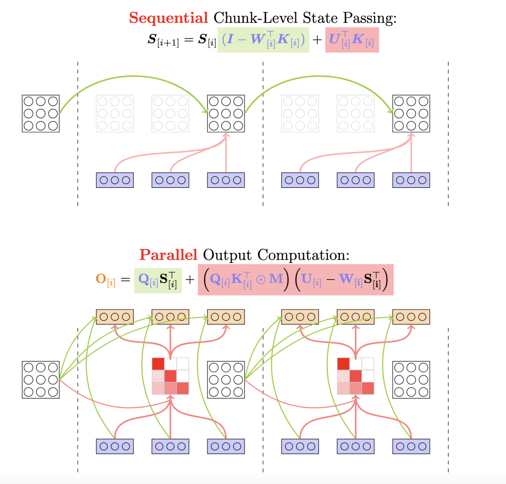
UT Transform Through the Lens of Graph Theory
The chunkwise parallel form transforms most of DeltaNet’s operations into efficient matrix multiplications similar to linear attention. However, there’s a key computational bottleneck: the recursive construction of update vectors \(\mathbf{U}_{[i]}\) and \(\mathbf{W}_{[i]}\). This motivates the need for the UT transform
In graph theory, for a weighted directed graph, the adjacency matrix \(\mathbf{A}\) captures direct connections - entry \(\mathbf{A}[i,j]\) represents the edge weight from node \(j\) to node \(i\). When we compute \((\mathbf{I} - \mathbf{A})^{-1}\), each entry \([i,j]\) gives the sum of weights of all possible paths from \(j\) to \(i\).
Looking at our recursive update equations:
\[\mathbf{w}_{[t]}^r = \beta_{[t]}^r \left(\mathbf{k}_{[t]}^r - \sum_{i=1}^{r-1} \mathbf{w}_{[t]}^i (\mathbf{k}_{[t]}^i)^\top\mathbf{k}_{[t]}^r \right)\] \[\mathbf{u}_{[t]}^r = \beta_{[t]}^r \left(\mathbf{v}_{[t]}^r - \sum_{i=1}^{r-1} \mathbf{u}_{[t]}^i (\mathbf{k}_{[t]}^i)^\top\mathbf{k}_{[t]}^r \right)\]These form a weighted directed graph where:
- Nodes represent sequence positions
- Directed edges connect position \(i\) to \(r\) where \(i < r\) (causal dependency)
- Edge weights \(-\beta_{[t]}^r\mathbf{k}_{[t]}^{i\top}\mathbf{k}_{[t]}^r\) encode interactions through key similarity and learning rate
This graph structure can be represented by the adjacency matrix, which could be computed efficiently:
\[\mathbf{A}_{[t]} = \operatorname{tril}(-\operatorname{diag}(\boldsymbol{\beta}_{[t]})\mathbf{K}_{[t]} \mathbf{K}_{[t]}^\top,-1)\]Since \(\mathbf{A}_{[t]}\) is strictly lower triangular, \((\mathbf{I} - \mathbf{A}_{[t]})\) is also lower triangular with ones on the diagonal. This special structure allows us to efficiently compute its inverse through forward substitution:
\[\mathbf{T}_{[t]} = \left(\mathbf{I} - \mathbf{A}_{[t]}\right)^{-1}\]This avoids the need for general matrix inversion, making the computation much more efficient. After obtaining \(\mathbf{T}_{[t]}\), which captures all accumulated influence paths between positions, we proceed with the final multiplication:
\[\mathbf{W}_{[t]} = \mathbf{T}_{[t]} \operatorname{diag}(\boldsymbol{\beta}_{[t]})\mathbf{K}_{[t]}, \quad \mathbf{U}_{[t]}=\mathbf{T}_{[t]}\operatorname{diag}(\boldsymbol{\beta}_{[t]})\mathbf{V}_{[t]}\]Applies these accumulated influences to compute our updates in a hardware-efficient form.
Speed comparison
We implemented both the recurrent and chunkwise parallel versions of DeltaNet using Triton. Our experiments compare their performance across different sequence lengths (\(L\)) and head dimensions (\(d_{\text{head}}\)), with a fixed model dimension \(d=2048\). To ensure fair comparison across configurations, we kept the total sequence elements constant at 16,384 by adjusting batch sizes accordingly.
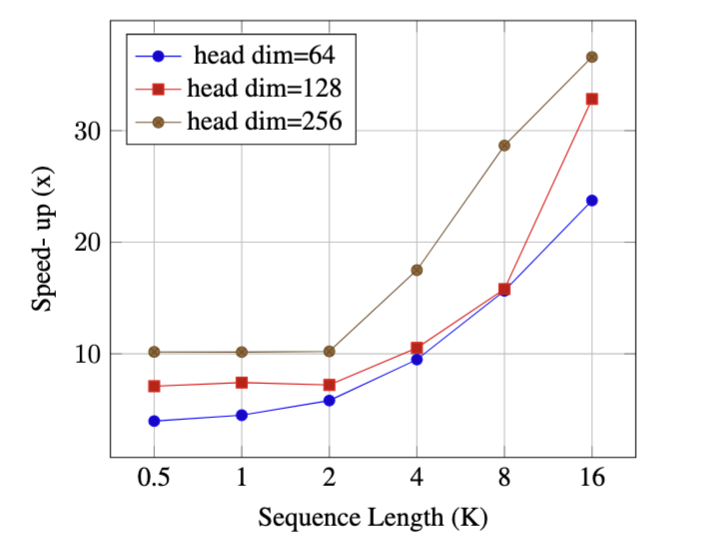
As we can see in the figure above, our chunkwise parallel approach consistently outperforms the recurrent baseline. More importantly, this performance advantage grows more pronounced under two key conditions: as sequences get longer and as head dimensions increase. To understand why, let’s examine two fundamental limitations of recurrent implementations that our approach addresses.
The first limitation concerns parallelism strategy. Recurrent implementations process sequences step-by-step, relying primarily on two sources of parallelism to keep GPU cores busy: the batch dimension (processing multiple sequences simultaneously) and the head dimension (computing multiple attention heads in parallel). While this strategy worked well with moderate sequence lengths and larger batch sizes, it faces challenges in modern training scenarios. Today’s models increasingly work with longer sequences or larger model parameters, often necessitating smaller batch sizes for memory efficiency. This shift was notably highlighted in the FlashAttention2 paper
The second limitation relates to hardware utilization. Modern GPUs include specialized tensor cores designed to accelerate matrix multiplication operations, offering up to 16x speedup for half-precision computations compared to other operations with equivalent FLOP counts. Recurrent implementations, despite requiring fewer total FLOPs, struggle to effectively leverage these hardware accelerators. This becomes particularly problematic with larger head dimensions, which are often necessary for tasks requiring substantial memory capacity (like in-context retrieval). Our chunkwise implementation, in contrast, restructures the computation to maximize use of tensor cores, achieving better real-world performance despite higher theoretical FLOP counts. This performance analysis illustrates a crucial principle in modern hardware-efficient deep learning: raw FLOP counts don’t always translate directly to wall-clock time. The ability to leverage specialized hardware accelerators and maintain high GPU utilization often matters more than theoretical operation counts. Our chunkwise implementation succeeds by aligning the computation with these hardware realities.
Finally, we compare DeltaNet’s training throughput against other models at the 1.3B parameter scale.
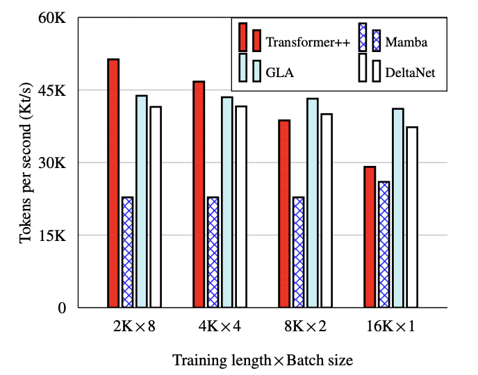
DeltaNet achieves competitive throughput, running only slightly slower than GLA (Gated Linear Attention). This small performance gap is a reasonable trade-off for DeltaNet’s more expressive transition matrices.